Lasers and Diffraction

Supervisor : J. Roussel

Elements of diffraction

Diffraction refers to various phenomena that occur when a wave encounters an obstacle or a slit. It is defined as the bending of light around the corners of an obstacle or aperture into the region of the geometrical shadow of the obstacle. These characteristic behaviors are exhibited when a wave encounters an obstacle or an aperture that is comparable in size to its wavelength.

The scalar theory of diffraction was established by Augustin Fresnel. The Fraunhofer diffraction is an approximation which applies to the far field; that is when the diffraction pattern is viewed at a long distance from the diffracting aperture.

The theoretical results will be provided without demonstration.

First example: diffraction by a single-slit

Consider a single slit which is illuminated by a light plane wave (a laser beam is a good approximation). The intensity profile of the diffracted light can be calculated using the Fraunhofer diffraction equation as \[ I(\theta)=I_{0}\,\text{sinc}\left(\dfrac{\pi\,\ell\,\sin \theta}{\lambda}\right)^{2} \quad\text{with}\quad \text{sinc}(x)=\frac{\sin x}{x} \] where

• $I(\theta)$ is the intensity in a direction given by the angle $\theta$;
• $\ell$ is the width of the slit;
• $\lambda$ is the wavelength of the plane wave.

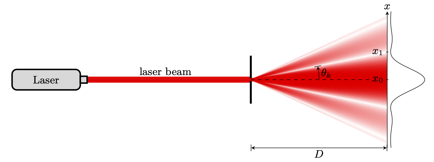
Let us compute the minima of the intensity pattern (dark fringes corresponding to destructive interference), defined by $I(\theta)=0$. This gives \[ \dfrac{\pi\,\ell\,\sin \theta}{\lambda}=k\,\pi \quad\Longrightarrow\quad \sin\theta_k=k\frac{\lambda}{\ell} \quad\text{with}\quad k\in \mathbb{Z^*} \]

If the interference pattern is recorded by a CCD sensor at a distance $D$, these minima correspond to the positions $x_k$ given by \[ \tan\theta_k=\frac{x_k-x_0}{D} \] where $x_0$ is the position of the central maximum. If we assume small angles, we have $\tan \theta_k\simeq \sin\theta_k$ and we find \begin{equation} \boxed{x_{k}=k\frac{\lambda D}{\ell}+x_0} \label{eq:TP2Minima} \end{equation}

Second example: diffraction by a circular aperture

When a plane wave falls on a plate with a circular hole, this aperture diffracts light and produces a divergent beam. The narrower hole is, the more divergent the beam is. The intensity profile shows circular dark fringes. The central spot is named the Airy disc and its diameter is given by \begin{equation} \boxed{\phi=a\frac{\lambda D}{d}} \label{eq:TP2_formule_airy} \end{equation} where $d$ is the diameter of the hole and $a$ is a numerical constant that you will have to measure.

Equipment

CCD sensor

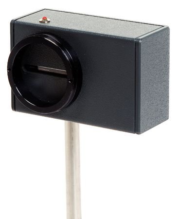
The intensity profile is recorded by horizontal CCD sensor directly interfaced with a PC computer. The sensor is composed of 2048 pixels, 14 μm in width. The optical device fixed on an optical bench can be horizontally and vertically adjusted.

The sensor is very sensitive, and it is often necessary to attenuate the intensity of the beam in order to avoid saturation. This is why a filter is screwed on the sensor. To reduce the intensity further, two crossed polarizers (Malus's law) can be used.

Once adjusted, luminous pictures can be sampled and operated with the help of software, named CALIENS™.

CALIENS software

The software displays in real time the distribution of the light intensity along the CCD sensor (activate ACQUISITION CONTINUE). To record the signal, activate the button ACQUISITION SIMPLE. Then, you can zoom in and display cursors.

The figure below shows a screenshot of a CALIENS window.

Manipulations

SAFETY INSTRUCTIONS

• Before turning on the laser, be sure that it is pointed away from yourself and others.
• Never look directly into the laser.
• Never direct the laser beam at another person.

Divergence of the laser beam

For the experiments, we use a 1 mW HeNe laser, which emits in the red part of the visible spectrum.

Beam profile — The profile intensity of a laser is Gaussian: \begin{equation} \boxed{ I(r)=I_\text{max}\,\mathrm{e}^{-2r^2/w^2} } \label{tp_diffraction_eq1} \end{equation} where $r$ is the radial distance from the centre of the axis beam. The $w$ parameter measures the beam radius.

Beam divergence — The beam diameter \(2w(x)\) increase along the optical path because of the beam divergence. We can calculate the angle \(\theta\) from the variation of \(w(x)\).

1. Place the laser and the CCD sensor on the optical bench. Fix the CCD sensor (with the filter) at x = 70 cm. Turn on the laser.
2. Turn on the CALIENS software and adjust filtering to medium level (Parametres ▶ Acquisition ▶ Filtre).
3. Carefully align (horizontally and vertically) the laser beam with the center of the sensor to obtain an optimum signal. Cross the polarisers to reduce the intensity if necessary. Once adjusted, record the signal.
4. Put an horizontal cursor at the top of the signal ($I_\text{max}$) and at $I_\text{max}\,\mathrm{e}^{−2}$. Deduce the $w$ parameter using \eqref{tp_diffraction_eq1}.

Call the teacher for verification.

5. Repeat the measure for x = 110, 150 and 190 cm. Plot \(w\) versus \(x\) then determine the beam divergence of the laser (express the result in in milli-radians).

Diffraction by a single slit and circular aperture

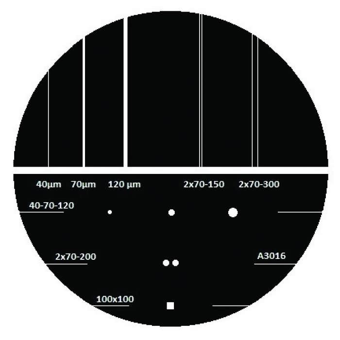
For these manipulations, use the token on which different diffracting apertures are lithographed (see figure opposite).

Diffraction by a single slit — We analyse the diffraction of the laser beam by a single slit of $\ell=120\,\mathrm{\mu m}$ in width.

1. Set the slit on the optical bench at 1 m from the laser and carefully align (horizontally and vertically) the laser beam with the center of the slit.
2. Place the CCD at the end of the optical bench and measure the distance $D$.
   NB: CCD sensor is 15 mm offset from the support axis.
3. Acquire the intensity profile of diffracted light. If the intensity is too low, increase Sensitivity. Accurately measure the $x_k$ position of the minima.
4. Fill in a table in REGRESSI™, with $k$ and $x_k$ data. Then, plot $x_k$ versus $k$ and choose the model to adjust with your data.
5. Is the \eqref{tp_diffraction_eq1} law verified ? Deduce $\lambda$ and compare with $\lambda^\text{tab}=632\,\mathrm{nm}$.

Diffraction by a circular aperture — In this experiment we explore the light diffracted by a circular hole with 120 μm diameter. The procedure is the same as before.

1. Carefully align (horizontally and vertically) the laser beam with the center of the hole with 120 μm diameter. You can illuminate the back of the hole with a lamp to adjust the laser spot over the hole.
2. Observe the diffraction pattern on a screen behind the hole and then observe the signal in CALIENS™. Identify the Airy disc and the rings.
3. In order to measure the Airy disc diameter, adjust the vertical position of the CCD sensor. Measure $\phi$, the Airy disc diameter (don’t forget to estimate uncertainty).
4. Determine the $a$ constant at a confidence level of 95%. Comment on your result.

★★★