
Speed of Light
Objectives : evaluate the speed of light, in different materials, using an optoelectronic device the size of a lab bench.
Prerequisite : refractive index, phase shifting.
A bit of history
In 1676 Cassini and Rømer made the first quantitative measurements of the speed of light. Cassini observed Jupiter's moons between 1666 and 1668, and discovered discrepancies in his measurements that, at first, he attributed to light having a finite speed. In 1672 Rømer went to Paris and continued observing Jupiter's satellites as Cassini's assistant. Rømer added his own observations to Cassini's and observed that times between eclipses (particularly those of Io) got shorter as the Earth approached Jupiter, and longer as the Earth moved farther away. Light seems to take about ten to eleven minutes to cross a distance equal to the half-diameter of the terrestrial orbit thus leading to a speed of light of about 220 000 km/s.

In 1728 James Bradley, an English physicist, estimated the speed of light in vacuum to be around \(301\,000~\mathrm{km.s^{-1}}\). He used stellar aberration to calculate the speed of light. Stellar aberration causes the apparent position of stars to change due to the motion of the Earth around the sun. Stellar aberration is approximately the ratio of the speed that the earth orbits the sun to the speed of light. He knew the speed of the Earth around the sun and he could also measure this stellar aberration angle. These two facts enabled him to calculate the speed of light in vacuum.
In 1849 Hippolyte Fizeau, a French physicist, shone a light between the teeth of a rapidly rotating toothed wheel. A mirror more than 5 miles away reflected the beam back through the same gap between the teeth of the wheel. There were over a hundred teeth in the wheel which rotated at hundreds of times a second; therefore a fraction of a second was easy to measure. By varying the speed of the wheel, it was possible to determine at what speed the wheel was spinning too fast for the light to pass through the gap between the teeth, to the remote mirror, and then back through the same gap. He knew how far the light traveled and the time it took. By dividing that distance by the time, he found the speed of light was \(313\,300~\mathrm{km.s^{-1}}\).
Leon Foucault, another French physicist, used a similar method to Fizeau's. A beam of light was shone towards a rotating mirror, then bounced back to a remote fixed mirror and then back to the first rotating mirror. Because the first mirror was rotating, the light finally bounced back at an angle slightly different from the angle it initially hit the mirror with. By measuring this angle, it was possible to measure the speed of light. His final measurement in 1862 determined that light traveled at \(299\,796~\mathrm{km.s^{-1}}\).
In the early 1860s, James Clerk Maxwell showed that, according to the theory of electromagnetism he was working on, light is an electromagnetic wave that propagates in vacuum at a speed equal to \(c=1/\sqrt{\varepsilon_0\mu_0}\). Afterwards, Albert Einstein, in 1905, postulated the invariance of the speed of light in vacuum leading to special relativity.
Today, the speed of light in vacuum is fixed at \(c=299\,792\,458~\mathrm{m.s^{-1}}\) (no uncertainty!) and tied to the definition of the meter.
(see https://www1.bipm.org/utils/common/pdf/si_brochure_8.pdf p.112)
Theory
How to measure the speed of light on a lab bench?
Summary.
It takes time to travel from a source to a receiver (distant from \(L\)). Thus the peak of a sine wave is delayed between source and receiver:
\[
\Delta{t}=\dfrac{L}{c}
\qquad\Leftrightarrow\qquad
\boxed{\phi=2\pi\,f\,\dfrac{L}{c}}\hspace{0.5em}\heartsuit
\]
Light of speed \(c\) is deduced by measuring \(f\), \(L\) and \(\phi\).
In detail.
Visible light is an electromagnetic wave that oscillates at approximatively 1014 Hz. This is too fast so that we cannot directly measure a phase shift which would rapidly change over distances as small as 1 µm (not measurable on a lab bench).
The technic consists in modulating the light emitted by a red LED at a lower frequency \(f_\mathrm{mod}=50.1\) MHz (yielding phase shifts over distances \(\simeq 1~\mathrm{m}\)). This frequency is yet not suitable for a classic oscilloscope but the phase shift can be obtained via mixing the signal at \(f_\mathrm{mod}\) with a sine wave at a frequency \(f_\mathrm{ref}\) very close to \(f_\mathrm{mod}\). See figure below.

The resulting signals contain two partials with a high and a low frequency. The high frequency can not be detected by the oscilloscope because it is out of its bandwidth. Let us see how the phase difference is kept during the operation:
- The emitting diode signal varies (=is modulated) around the mean value A: \[s_{\mathrm{e}}(t)=A+B\cos(2\pi f_{\mathrm{mod}}t)\]
- The receiving diode produces a signal proportional (\(\alpha\)) to \(s_{\mathrm{e}}\), with a delay due to the distance (\(L/c\)): \[ s_{\mathrm{r}}(t) =\alpha\times s_{e}(t-L/c) = \alpha A+\alpha B\cos\left(2\pi f_{\mathrm{mod}}t-\frac{2\pi f_{\mathrm{mod}}L}{c}\right) \]
Both signals are multiplied by a reference sine wave (\(f_{\mathrm{ref}}=50{.}05\) MHz): \[ \left. \begin{array}{c} \alpha A+\alpha B\cos(2\pi f_{\mathrm{mod}}t+\phi)\\ \times\\ \cos(2\pi f_{\mathrm{ref}}t) \end{array} \right\}\: s(t)=\alpha A\cos(2\pi f_{\mathrm{ref}}t)+\alpha B\cos(2\pi f_{\mathrm{ref}}t).\cos(2\pi f_{\mathrm{mod}}t+\phi)\\ \] And with a pinch of trigonometry, \[ s(t) =\alpha A\cos(2\pi f_{\mathrm{ref}}t) +\frac{\alpha}{2}B \big[ \underbrace{\vphantom{\dfrac{1}{1}} \cos\left( 2\pi(f_{\mathrm{mod}}+f_{\mathrm{ref}})t+\phi\right)}_{\text{high frequency}} +\underbrace{\vphantom{\dfrac{1}{1}} \cos\left(2\pi(f_{\mathrm{mod}}-f_{\mathrm{ref}})t+\phi\right)}_{\text{low frequency}} \big] \] Since the o-scope bandwidth is limited to [0 ; 20 MHz], high frequencies are rejected:
- \(f_{\mathrm{mod}}+f_{\mathrm{ref}}\simeq\) 100 MHz disappears;
- \(f_{\mathrm{mod}}-f_{\mathrm{ref}}\simeq\) 50 kHz remains and is displayed on the oscilloscope.
Finally, on the X-channel: \[\quad\boxed{s_{X}=\dfrac{B}{2}[\cos(2\pi(f_{\mathrm{mod}}-f_{\mathrm{ref}})t)]}\]
and on the Y-channel: \[\quad\boxed{s_{Y}=\dfrac{\alpha B}{2}[\cos(2\pi(f_{\mathrm{mod}}-f_{\mathrm{ref}})t+\phi)]}\]
The phase information is preserved and leads to the speed of light \(c\). This method is called heterodyne detection (see https://en.wikipedia.org/wiki/Optical_heterodyne_detection).
How to measure a phase difference?
Signals \(\mathbf{s_X}\) and \(\mathbf{s_Y}\) over time

Method:
- Display both channels as a function of time.
- Scale each voltage channel so that each waveform fits in the display.
- Ground (zero) each channel separately and adjust the line to the center axis.
- Return to ac coupling.
- Pick a feature (peak or zero crossing for sinusoids) to base your time measurements on.
NB: the peak of a sinusoid is not affected by dc offsets but is harder to pinpoint than the zero crossing.
Measurement involves proportionality between \(\Delta{t}\) (smallest time difference between occurrences of the feature on the two waveforms) and \(\phi\): \[ \phi=2\pi\,\dfrac{\Delta{t}}{T} \] A larger spacing between occurrences of the feature provides a more accurate value.
Useful tip: if you can continuously adjust the time per division (=uncalibrate the time base), scale your waveforms so that half a period matches 9 divisions. As \(180/9=20\), a division now equals 20°!
Please note that thankfully the oscilloscope can measure a phase difference
just by pressing a few buttons:
MEAS ► more ► more ► \(\varphi\)
alt or chop mode?
On analog scopes, because there is only one electronic beam, multiple channels are displayed using either an alternate or chop mode.
- Alternate mode draws each channel alternately. Use this mode with medium to high speed signals, when the sec/div scale is set to 0.5 ms or faster.
- Chop mode causes the oscilloscope to draw small parts of each signal by switching back and forth between them. You typically use this mode with slow signals requiring sweep speeds of 1 ms per division or less.
Signals \(\mathbf{s_X}\) and \(\mathbf{s_Y}\) in XY-mode
Lissajous Method.
In XY-mode, the o-scope draws \(s_Y\) versus \(s_X\). This defines a parametric curve (Lissajous curve):
\[
\left\{
\begin{array}{rcl}
X(t) &=&a\cos(\omega t)\\
Y(t) &=&b\cos(\omega t+\phi)
\end{array}
\quad\text{with}\quad
\omega = 2\pi(f_{\mathrm{mod}}-f_{\mathrm{ref}})
\right.
\]
It is an ellipse equation, contained in a \(2a\times 2b\) rectangle. Its eccentricity \(e\) varies with \(\phi\).


Method:
- Set the oscilloscope to XY mode.
- Scale each voltage channel so that the ellipse fits in the display.
- Ground or zero each channel separately and adjust the line to the center (vertical or horizontal) axis of the display. (On analog scopes, you can ground both simultaneously and center the resulting dot.)
- Return to ac coupling to display the ellipse.
NB: A 0 or \(\pi\)-phase difference provides a more accurate measurement.
How to measure a refractive index?
The velocity \(v\) of light traveling through a material is lesser than in vacuum or air: \(v=c/n\). Therefore the delay between emitter and receiver is \[ \Delta{t} =\dfrac{d_\mathrm{air}}{c}+\dfrac{d_\mathrm{m}}{v} =\dfrac{d_\mathrm{air}}{c}+\dfrac{n\,d_\mathrm{m}}{c} \] \(d_\mathrm{air}\) is the total length of the light path in air. \(d_\mathrm{m}\) is the total length of the light path in the material. The phase difference becomes \[ \boxed{ \phi=\dfrac{2\pi f_{\mathrm{mod}}}{c}( d_\mathrm{air}+n\,d_\mathrm{m} ) } \hspace{0.5em}\heartsuit \]
Two measures are performed during the experiment.
- Place the mirrors immediately after the material (\(x_1\) position) and choose an appropriate phase difference by adjusting the
PHASEbutton on the Phywe generator. - Remove the material and slide away the mirrors until you get back the same chosen phase difference (\(x_2\) position).


Depending on the chosen layout, \[ \boxed{n=1+\dfrac{x_2-x_1}{\ell_\mathrm{m}}} \qquad\text{or}\qquad \boxed{n=1+2\,\dfrac{x_2-x_1}{\ell_\mathrm{m}}} \]
Tasks
Preparation
Principle of the experiment
Which order of magnitude of frequency is necessary to obtain a measurable phase shift on a lab bench?
Is this frequency compatible with an oscilloscope?
Use Python to draw a Lissajous curve as shown by an oscilloscope when two phase-shifted sinusoid inputs are applied in X-Y mode. Try different phase difference.
Measuring a refractive index
Demonstrate the formulae of the refractive indexes of plexiglas and water: \[ \boxed{n_\mathrm{p}=1+\dfrac{x_2-x_1}{\ell_\mathrm{m}}} \qquad\text{and}\qquad \boxed{n_\mathrm{w}=1+2\dfrac{x_2-x_1}{\ell_\mathrm{m}}} \] Express the uncertainty on \(n_\mathrm{p}\) and \(n_\mathrm{w}\).
Manipulations
Set-up
This is a crucial point of the experiment.
- The Phywe generator needs 10 minutes to warm.
- Put the mirrors 1 meter away from the generator.
- Tune the position of the first lens (vertically and laterally) so that you get the maximum of light on the first mirror (use a screen or a white sheet to check that).
- Then adjust the position of the second lens to focus the beam on the photoreceptor cell (look at the cell!).
- Finally fine tune the apparatus thanks to the screws on the mirrors. The sine waves on the scope must be as large as possible.
Light velocity in the air
Write down the value of \(f_\mathrm{mod}\) thanks to the frequency meter (which reads \(f_\mathrm{mod}/1000\)).
First method
- In XY-mode, find the distance between positions corresponding to \(\phi=0\) and \(\phi=180\)°.
- Deduce the speed of light along with its uncertainty.
Second method
- Seeing the sine waves on the oscilloscope, find the position of the mirrors when the phase difference equals \(\phi=90\)°.
- Start from scratch again to get four independent measurement (meaning unsettling the phase button, the lenses, etc).
- Use the Student's t-distribution to obtain \(c\) and its uncertainty.
Outcome
Compare the two speeds of light and conclude.
Measuring a refractive index
- Choose an appropriate phase difference.
- Measure \(x_1\) and \(x_2\) pour plexiglas block and the water-filled tube.
- Give the refractive indexes along with their uncertainty.
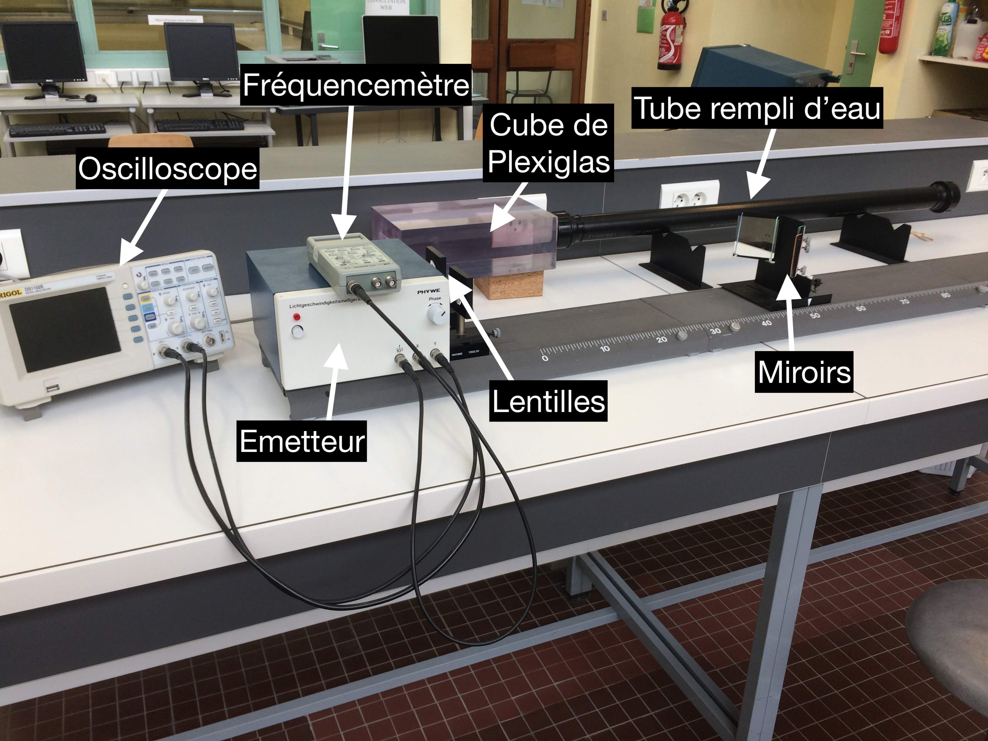
Matériel
- an oscilloscope analogique METRIX ;
- a frequency meter;
- a Phywe generator with a graduated rail, a pair of mirrors and lenses;
- a Plexiglas block and a water-filled tube.